sp.multirate

Module providing Multirate signal processing functionality. Largely based on MATLAB’s Multirate signal processing toolbox with consultation of Octave m-file source code.

Example Usage

downsample

>>> import numpy
>>> from sp import multirate
>>> x = numpy.arange(1, 11)
>>> multirate.downsample(x, 3)
array([ 1,  4,  7, 10])
>>> multirate.downsample(x, 3, phase=2)
array([3, 6, 9])

upsample

>>> import numpy
>>> from sp import multirate
>>> x = numpy.arange(1, 5)
>>> multirate.upsample(x, 3)
array([ 1.,  0.,  0.,  2.,  0.,  0.,  3.,  0.,  0.,  4.,  0.,  0.])
>>> multirate.upsample(x, 3, 2)
array([ 0.,  0.,  1.,  0.,  0.,  2.,  0.,  0.,  3.,  0.,  0.,  4.])

decimate

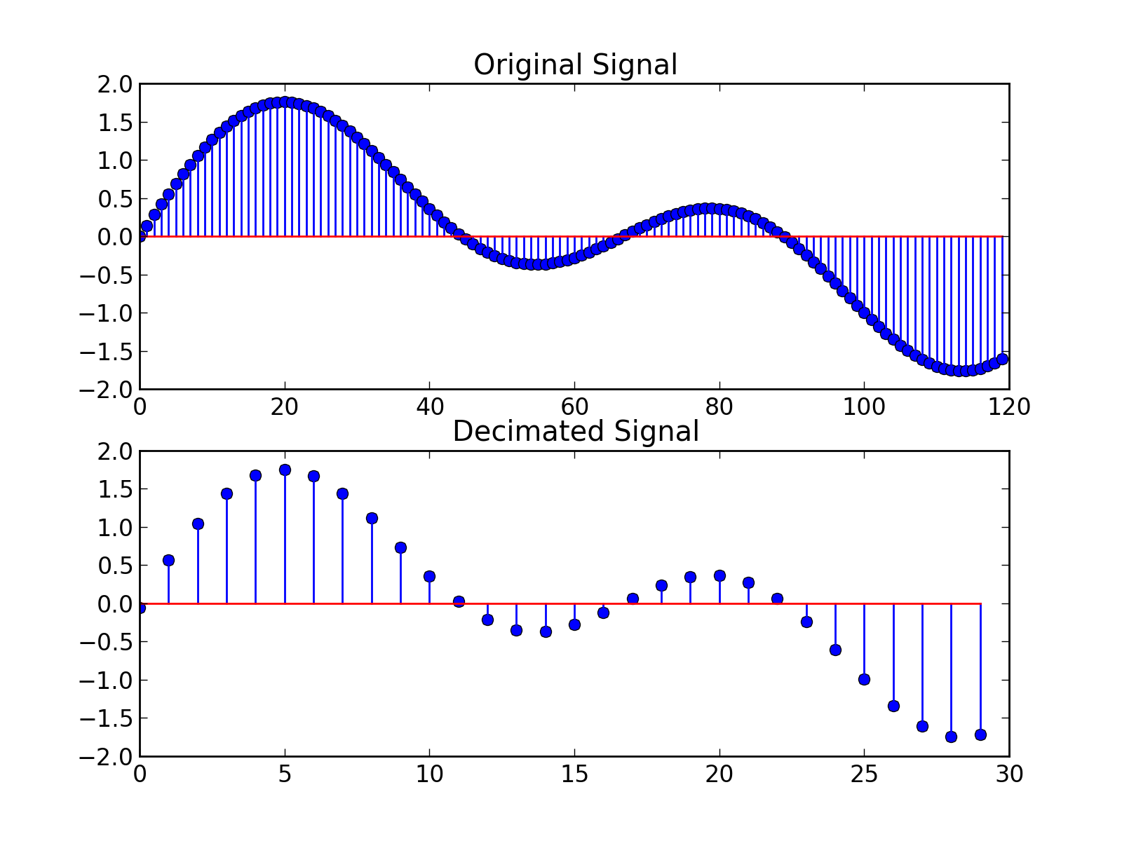
import numpy
import pylab
from sp import multirate
t = numpy.arange(0, 1, 0.00025)
x = numpy.sin(2*numpy.pi*30*t) + numpy.sin(2*numpy.pi*60*t)
y = multirate.decimate(x,4)
pylab.figure()
pylab.subplot(2, 1, 1)
pylab.title('Original Signal')
pylab.stem(numpy.arange(len(x[0:120])), x[0:120])
pylab.subplot(2, 1, 2)
pylab.title('Decimated Signal')
pylab.stem(numpy.arange(len(y[0:30])), y[0:30])
pylab.show()

(Source code, png, hires.png, pdf)

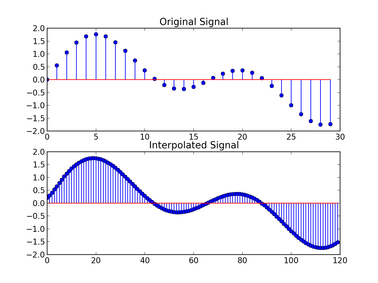
interp

import numpy
import pylab
from sp import multirate
t = numpy.arange(0, 1, 0.001)
x = numpy.sin(2*numpy.pi*30*t) + numpy.sin(2*numpy.pi*60*t)
y = interp(x,4)
pylab.figure()
pylab.subplot(2, 1, 1)
pylab.title('Original Signal')
pylab.stem(numpy.arange(len(x[0:30])), x[0:30])
pylab.subplot(2, 1, 2)
pylab.title('Interpolated Signal')
pylab.stem(numpy.arange(len(y[0:120])), y[0:120])
pylab.show()

(Source code, png, hires.png, pdf)

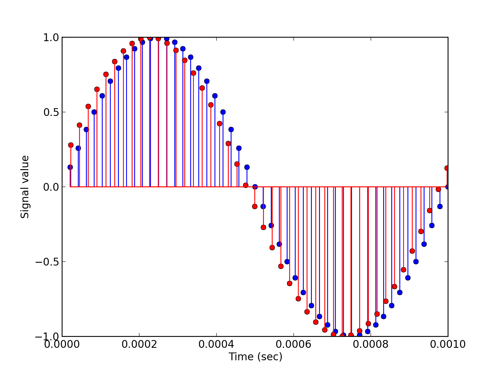
upfirdn

import numpy
import pylab
from sp import multirate
L = 147.0
M = 160.0
N = 24.0*L
h = signal.firwin(N-1, 1/M, window=('kaiser', 7.8562))
h = L*h
Fs = 48000.0
n = numpy.arange(0, 10239)
x  = numpy.sin(2*numpy.pi*1000/Fs*n)
y = multirate.upfirdn(x, h, L, M)
pylab.figure()
pylab.stem(n[1:49]/Fs, x[1:49])
pylab.stem(n[1:45]/(Fs*L/M), y[13:57], 'r', markerfmt='ro',)
pylab.xlabel('Time (sec)')
pylab.ylabel('Signal value')
pylab.show()

(Source code, png, hires.png, pdf)

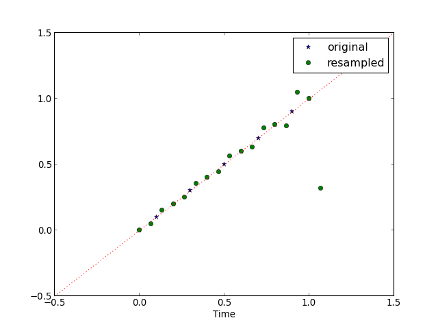
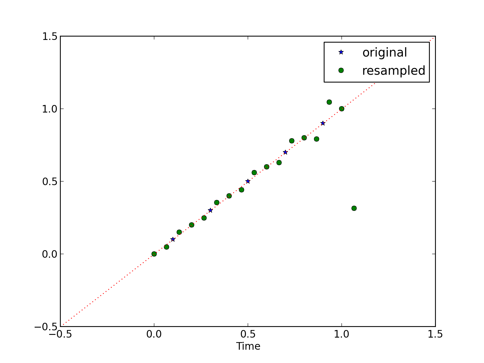
resample

import numpy
import pylab
from sp import multirate
fs1 = 10.0
t1 = numpy.arange(0, 1 + 1.0/fs1, 1.0/fs1)
x = t1
y = multirate.resample(x, 3, 2)
t2 = numpy.arange(0,(len(y)))*2.0/(3.0*fs1)
pylab.figure()
pylab.plot(t1, x, '*')
pylab.plot(t2, y, 'o')
pylab.plot(numpy.arange(-0.5,1.5, 0.01), numpy.arange(-0.5,1.5, 0.01), ':')
pylab.legend(('original','resampled'), numpoints=1)
pylab.xlabel('Time')
pylab.show()

(Source code, png, hires.png, pdf)

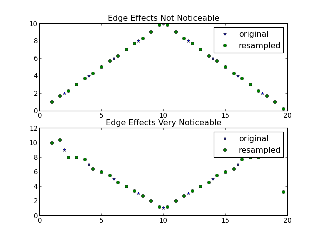
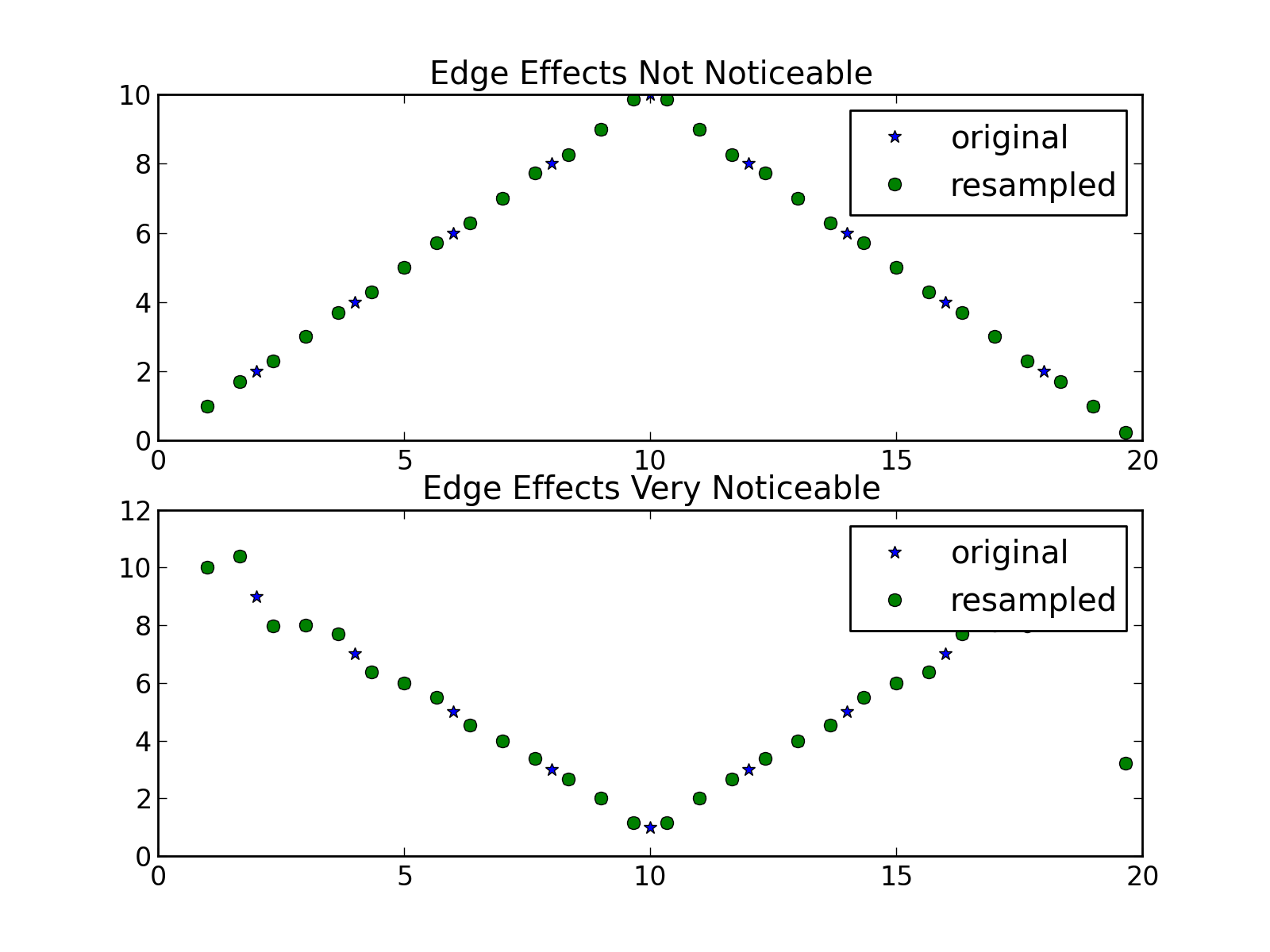
import numpy
import pylab
from sp import multirate
x = numpy.hstack([numpy.arange(1,11), numpy.arange(9,0,-1)])
y = multirate.resample(x,3,2)
pylab.figure()
pylab.subplot(2, 1, 1)
pylab.title('Edge Effects Not Noticeable')
pylab.plot(numpy.arange(19)+1, x, '*')
pylab.plot(numpy.arange(29)*2/3.0 + 1, y, 'o')
pylab.legend(('original', 'resampled'), numpoints=1)
x = numpy.hstack([numpy.arange(10, 0, -1), numpy.arange(2,11)])
y = multirate.resample(x,3,2)
pylab.subplot(2, 1, 2)
pylab.plot(numpy.arange(19)+1, x, '*')
pylab.plot(numpy.arange(29)*2/3.0 + 1, y, 'o')
pylab.title('Edge Effects Very Noticeable')
pylab.legend(('original', 'resampled'), numpoints=1)
pylab.show()

(Source code, png, hires.png, pdf)

See the individual methods below for further details.

Functions

sp.multirate.downsample(s, n, phase=0)

Decrease sampling rate by integer factor n with included offset phase.

sp.multirate.upsample(s, n, phase=0)

Increase sampling rate by integer factor n with included offset phase.

sp.multirate.decimate(s, r, n=None, fir=False)

Decimation - decrease sampling rate by r. The decimation process filters the input data s with an order n lowpass filter and then resamples the resulting smoothed signal at a lower rate. By default, decimate employs an eighth-order lowpass Chebyshev Type I filter with a cutoff frequency of 0.8/r. It filters the input sequence in both the forward and reverse directions to remove all phase distortion, effectively doubling the filter order. If ‘fir’ is set to True decimate uses an order 30 FIR filter (by default otherwise n), instead of the Chebyshev IIR filter. Here decimate filters the input sequence in only one direction. This technique conserves memory and is useful for working with long sequences.

sp.multirate.interp(s, r, l=4, alpha=0.5)

Interpolation - increase sampling rate by integer factor r. Interpolation increases the original sampling rate for a sequence to a higher rate. interp performs lowpass interpolation by inserting zeros into the original sequence and then applying a special lowpass filter. l specifies the filter length and alpha the cut-off frequency. The length of the FIR lowpass interpolating filter is 2*l*r+1. The number of original sample values used for interpolation is 2*l. Ordinarily, l should be less than or equal to 10. The original signal is assumed to be band limited with normalized cutoff frequency 0=alpha=1, where 1 is half the original sampling frequency (the Nyquist frequency). The default value for l is 4 and the default value for alpha is 0.5.

sp.multirate.upfirdn(s, h, p, q)

Upsample signal s by p, apply FIR filter as specified by h, and downsample by q. Using fftconvolve as opposed to lfilter as it does not seem to do a full convolution operation (and its much faster than convolve).

sp.multirate.resample(s, p, q, h=None)

Change sampling rate by rational factor. This implementation is based on the Octave implementation of the resample function. It designs the anti-aliasing filter using the window approach applying a Kaiser window with the beta term calculated as specified by [2].

Ref [1] J. G. Proakis and D. G. Manolakis, Digital Signal Processing: Principles, Algorithms, and Applications, 4th ed., Prentice Hall, 2007. Chap. 6

Ref [2] A. V. Oppenheim, R. W. Schafer and J. R. Buck, Discrete-time signal processing, Signal processing series, Prentice-Hall, 1999