sp.firwin

Module to design window based fir filter and analyse the frequency response of fir filters.

This implementation is largely based on Chapter 16 of The Scientist and Engineer’s Guide to Digital Signal Processing Second Edition.

Example Usage

Building a Lowpass Filter

import numpy
import pylab

from sp import firwin

f0 = 20 #20Hz
ts = 0.01 # i.e. sampling frequency is 1/ts = 100Hz
x = numpy.arange(-10, 10, ts)
signal = (numpy.cos(2*numpy.pi*f0*x) + numpy.sin(2*numpy.pi*2*f0*x) +
            numpy.cos(2*numpy.pi*0.5*f0*x) + numpy.cos(2*numpy.pi*1.5*f0*x))

#build filter
#Low pass
M = 100 #number of taps in filter
fc = 0.25 #i.e. normalised cutoff frequency 1/4 of sampling rate i.e. 25Hz
lp = firwin.build_filter(M, fc, window=firwin.blackman)

#filter the signal
filtered = numpy.convolve(signal, lp)

#plotting
pylab.figure()
pylab.subplot(3,1,1)
pylab.title('Original Spectrum')
pylab.xlabel('Normalised Frequency')
firwin.plot_fft(signal)
pylab.subplot(3,1,2)
pylab.title('Filter Frequency Response')
pylab.xlabel('Normalised Frequency')
firwin.plot_fft(lp)
#window and fft
pylab.subplot(3,1,3)
pylab.title('Filtered Spectrum')
pylab.xlabel('Normalised Frequency')
firwin.plot_fft(firwin.hamming(len(filtered))[:-1]*(filtered))
pylab.subplots_adjust(hspace = 0.6)
pylab.show()

(Source code, png, hires.png, pdf)

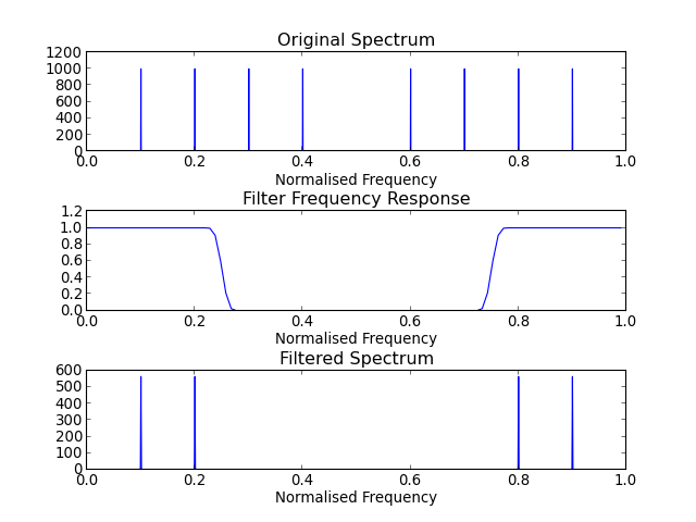
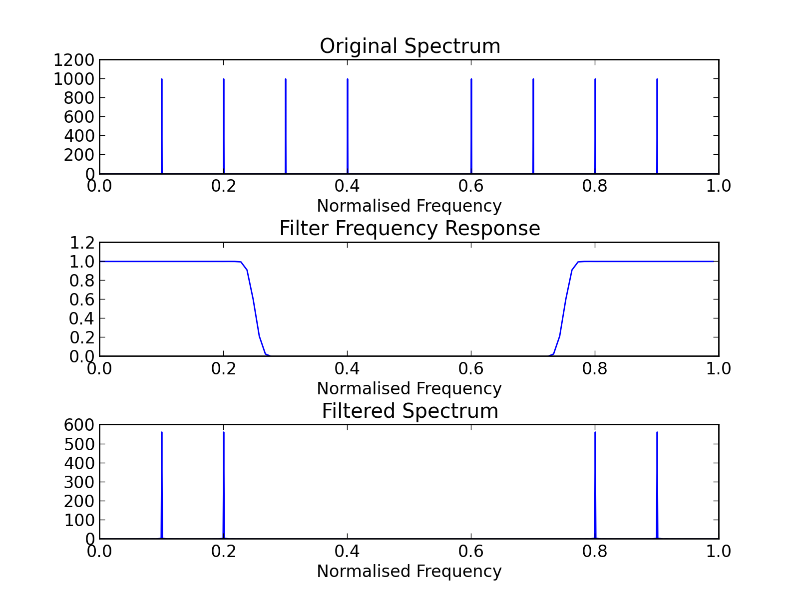
Building a Highpass Filter

import numpy
import pylab

from sp import firwin

f0 = 20 #20Hz
ts = 0.01 # i.e. sampling frequency is 1/ts = 100Hz
x = numpy.arange(-10, 10, ts)
signal = (numpy.cos(2*numpy.pi*f0*x) + numpy.sin(2*numpy.pi*2*f0*x) +
            numpy.cos(2*numpy.pi*0.5*f0*x) + numpy.cos(2*numpy.pi*1.5*f0*x))

#build filter
#First build a Lowpass filter
M = 100 #number of taps in filter
fc = 0.25 #i.e. normalised cutoff frequency 1/4 of sampling rate i.e. 25Hz
lp = firwin.build_filter(M, fc, window=firwin.blackman)
#next build Highpass filter by shifting frequency domain
shift = numpy.cos(2*numpy.pi*0.5*numpy.arange(M + 1))
hp = lp*shift

#filter the signal
filtered = numpy.convolve(signal, hp)

#plotting
pylab.figure()
pylab.subplot(3,1,1)
pylab.title('Original Spectrum')
pylab.xlabel('Normalised Frequency')
firwin.plot_fft(signal)
pylab.subplot(3,1,2)
pylab.title('Filter Frequency Response')
pylab.xlabel('Normalised Frequency')
firwin.plot_fft(hp)
#window and fft
pylab.subplot(3,1,3)
pylab.title('Filtered Spectrum')
pylab.xlabel('Normalised Frequency')
firwin.plot_fft(firwin.hamming(len(filtered))[:-1]*(filtered))
pylab.subplots_adjust(hspace = 0.6)
pylab.show()

(Source code, png, hires.png, pdf)

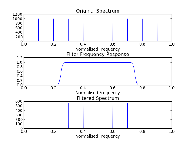
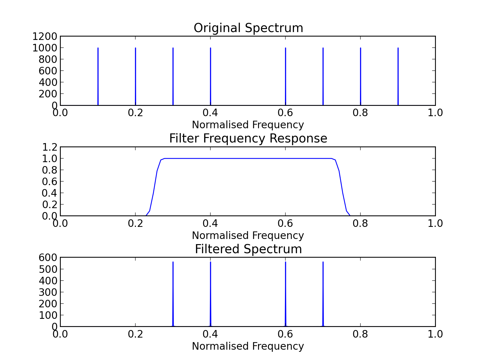
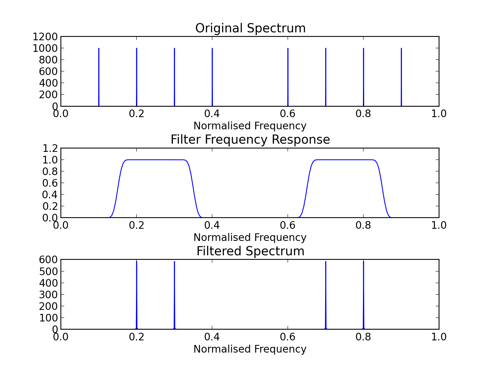
Building a Bandpass Filter

import numpy
import pylab

from sp import firwin

f0 = 20 #20Hz
ts = 0.01 # i.e. sampling frequency is 1/ts = 100Hz
x = numpy.arange(-10, 10, ts)
signal = (numpy.cos(2*numpy.pi*f0*x) + numpy.sin(2*numpy.pi*2*f0*x) +
            numpy.cos(2*numpy.pi*0.5*f0*x) + numpy.cos(2*numpy.pi*1.5*f0*x))

#build filter
#first need a low-pass with fc 0.35
M = 100 #number of taps in filter
fc = 0.35
lp = firwin.build_filter(M, fc, window=firwin.blackman)
shift = numpy.cos(2*numpy.pi*0.5*numpy.arange(M + 1))
hp = lp*shift
#now we can create the bandpass filter by convolution
bp = numpy.convolve(lp, hp)

#filter the signal
filtered = numpy.convolve(signal, bp)

#plotting
pylab.figure()
pylab.subplot(3,1,1)
pylab.title('Original Spectrum')
pylab.xlabel('Normalised Frequency')
firwin.plot_fft(signal)
pylab.subplot(3,1,2)
pylab.title('Filter Frequency Response')
pylab.xlabel('Normalised Frequency')
firwin.plot_fft(bp)
#window and fft
pylab.subplot(3,1,3)
pylab.title('Filtered Spectrum')
pylab.xlabel('Normalised Frequency')
firwin.plot_fft(firwin.hamming(len(filtered))[:-1]*(filtered))
pylab.subplots_adjust(hspace = 0.6)
pylab.show()

(Source code, png, hires.png, pdf)

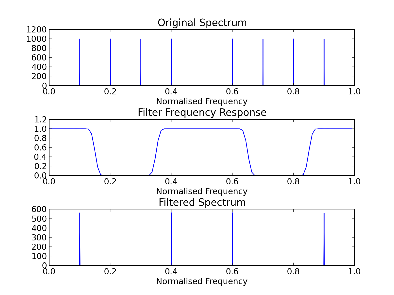
Building a Bandstop Filter

import numpy
import pylab

from sp import firwin

f0 = 20 #20Hz
ts = 0.01 # i.e. sampling frequency is 1/ts = 100Hz
x = numpy.arange(-10, 10, ts)
signal = (numpy.cos(2*numpy.pi*f0*x) + numpy.sin(2*numpy.pi*2*f0*x) +
            numpy.cos(2*numpy.pi*0.5*f0*x) + numpy.cos(2*numpy.pi*1.5*f0*x))

#build filter
#first need a low-pass with fc 0.15
M = 100 #number of taps in filter
fc = 0.15
lp = firwin.build_filter(M, fc, window=firwin.blackman)
#next need a high-pass
shift = numpy.cos(2*numpy.pi*0.5*numpy.arange(M + 1))
hp = lp*shift
#now we can create the bandstop filter by adding the two impulse responses
bs = lp + hp

#filter the signal
filtered = numpy.convolve(signal, bs)

#plotting
pylab.figure()
pylab.subplot(3,1,1)
pylab.title('Original Spectrum')
pylab.xlabel('Normalised Frequency')
firwin.plot_fft(signal)
pylab.subplot(3,1,2)
pylab.title('Filter Frequency Response')
pylab.xlabel('Normalised Frequency')
firwin.plot_fft(bs)
#window and fft
pylab.subplot(3,1,3)
pylab.title('Filtered Spectrum')
pylab.xlabel('Normalised Frequency')
firwin.plot_fft(firwin.hamming(len(filtered))[:-1]*(filtered))
pylab.subplots_adjust(hspace = 0.6)
pylab.show()

(Source code, png, hires.png, pdf)

See the individual methods below for further details.

Functions

sp.firwin.blackman(M)

Return an M + 1 point symmetric point hamming window.

sp.firwin.build_filter(M, fc, window=None)

Construct filter using the windowing method for filter parameters M number of taps, cut-off frequency fc and window. Window defaults to None i.e. a rectangular window.

sp.firwin.hamming(M)

Return an M + 1 point symmetric hamming window.

sp.firwin.plot_fft(x, style='b')

Convenience routine for plotting fft’s of signal with normalised frequency axis.

sp.firwin.sinc_filter(M, fc)

Return an M + 1 point symmetric point sinc kernel with normalised cut-off frequency fc 0->0.5.