sp.gauss

Module providing functionality surrounding gaussian function.

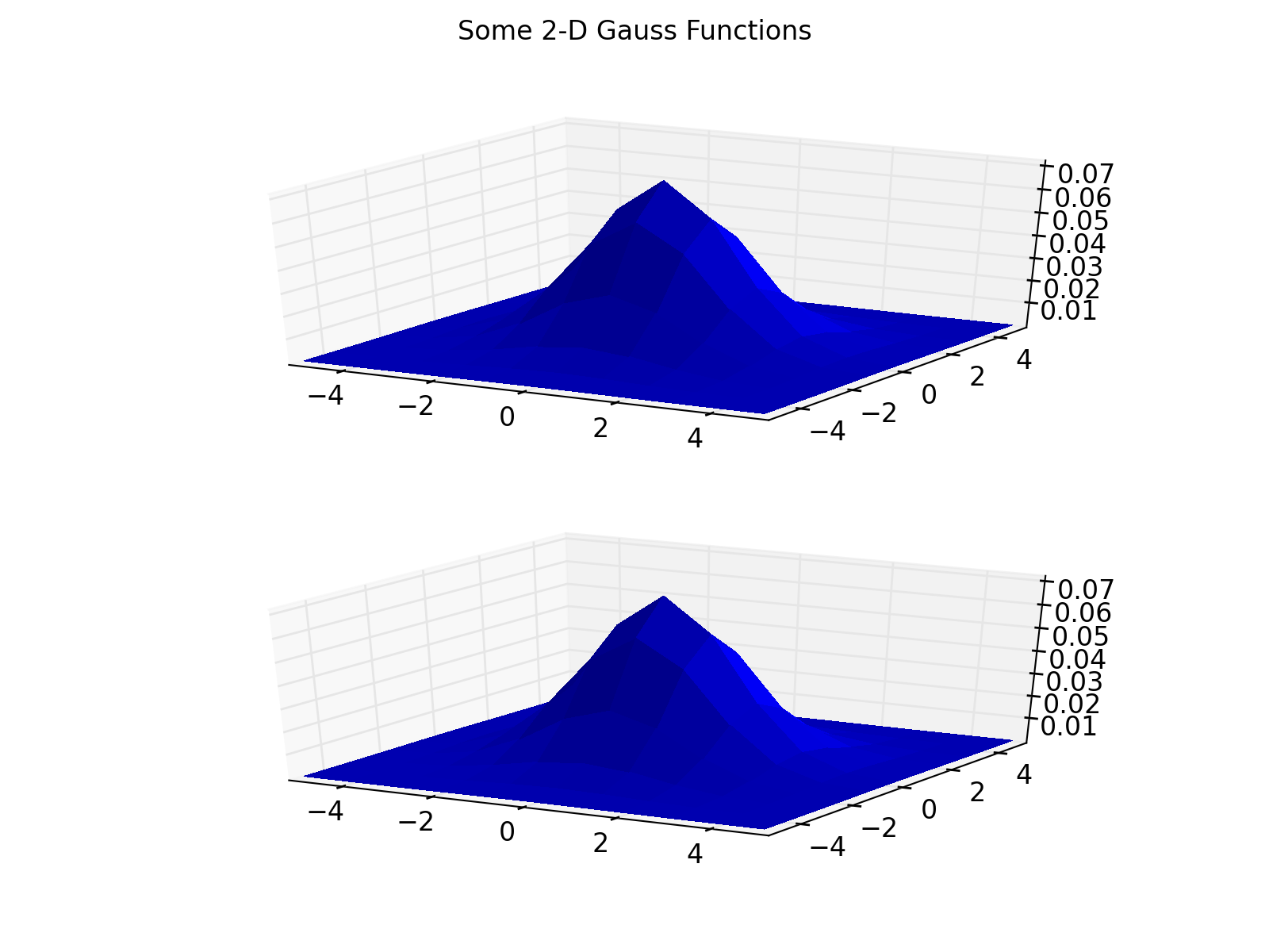
Example Usage

fspecial_gauss / gaussian2

from mpl_toolkits.mplot3d.axes3d import Axes3D
import pylab
import numpy
from sp import gauss
size = 11
sigma = 1.5
x, y = numpy.mgrid[-size//2 + 1:size//2 + 1, -size//2 + 1:size//2 + 1]

fig = pylab.figure()
fig.suptitle('Some 2-D Gauss Functions')
ax = fig.add_subplot(2, 1, 1, projection='3d')
ax.plot_surface(x, y, gauss.fspecial_gauss(size, sigma), rstride=1,
                cstride=1, linewidth=0, antialiased=False, cmap=pylab.jet())
ax = fig.add_subplot(2, 1, 2, projection='3d')
ax.plot_surface(x, y, gauss.gaussian2(size, sigma), rstride=1, cstride=1,
                linewidth=0, antialiased=False, cmap=pylab.jet())
pylab.show()

(Source code, png, hires.png, pdf)

See the individual methods below for further details.

Functions

sp.gauss.gaussian2(size, sigma)

Returns a normalized circularly symmetric 2D gauss kernel array

f(x,y) = A.e^{-(x^2/2*sigma^2 + y^2/2*sigma^2)} where

A = 1/(2*pi*sigma^2)

as define by Wolfram Mathworld http://mathworld.wolfram.com/GaussianFunction.html

sp.gauss.fspecial_gauss(size, sigma)

Function to mimic the ‘fspecial’ gaussian MATLAB function